Motivation

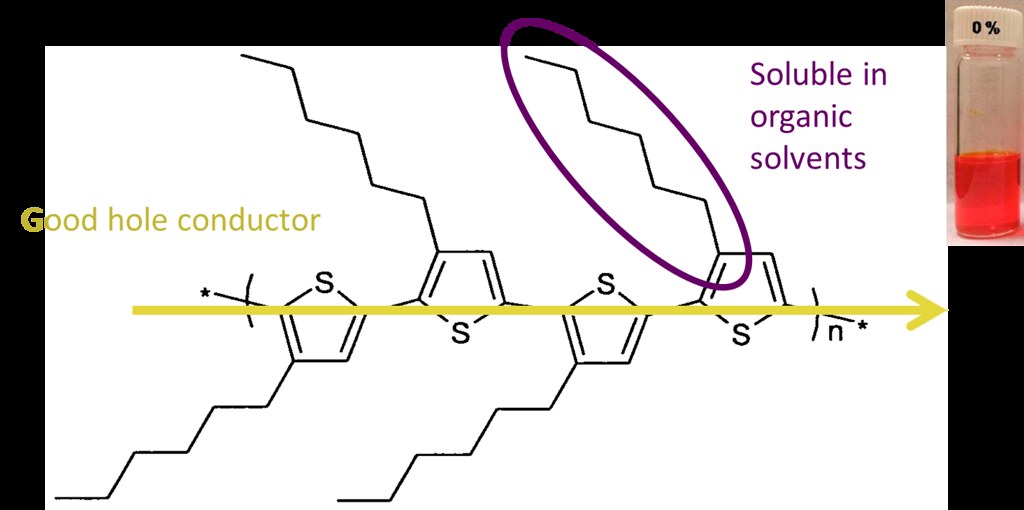
In order to reliably fabricate organic electronic devices, we must understand the quantitative relationship between their structure and their electronic properties. One widely studied system is that of poly-3-hexylthiophene (P3HT), a solution-processable polymeric semiconductor, and its charge carrier mobility in field effect transistors.

P3HT has a backbone with good hole conductor properties and side chains that make it soluble in organic solvents.

The crystal structure of P3HT has been thoroughly established in the extensive literature on the material:

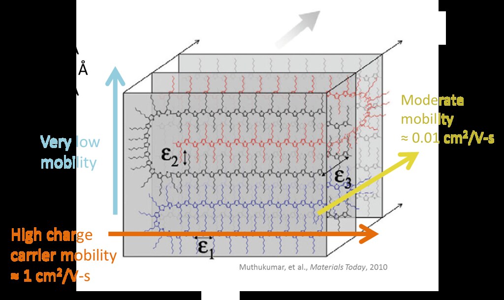
(a) (1 0 0) direction: alkyl stacking; (0 1 0): pi-stacking; (0 0 1): chain backbone (b) Face-on orientation, (c) edge-on orientation

Molecular Dynamics Simulations depict the ideal alkyl and pi-stacking conformations. Charge transport is fastest along the extended chain backbone (0 0 1) and pi-stacked directions (0 1 0). It is almost negligible for the purposes of this study, where our data is 2-dimensional. However, the measured hole mobility of a macro-scale film is usually orders of magnitude lower than that of the crystalline state.

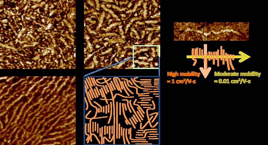
P3HT forms nanofibers during processing whose lengths correspond to the (0 1 0)/pi-stacking direction. The nanofibers register as regions with greater hardness/crystallinity in tapping-mode Atomic Force Microscopy (AFM) images:

Goal

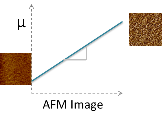
Our goal is to quantify the structure at the top layer of the P3HT thin film transistors, as represented by AFM images and to construct structure-property relationship µ = f(microstructure), where µ is hole mobility.

Data

The Reichmanis Group in ChBE performs studies on P3HT structure evolution during processing. They have a substantial collection of Atomic Force Microscopy (AFM) data paired with field-effect mobility measurements for P3HT thin film at a wide range of processing conditions. Twenty such AFM images and their paired mobility will be used for this study.

Approach

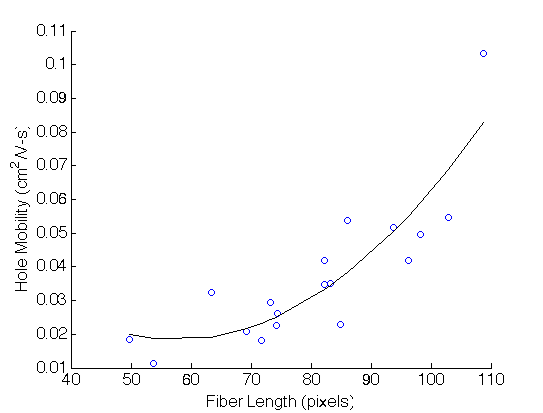
Simply by inspection, we can choose to regress against average fiber length and obtain a fit with a 2nd order polynomial.(Detailed for obtained the fiber lengths will be discussed in more detail in the method section)

However, many more potentially important features exist: - Orientation - Area fraction - Fiber density

Therefore we needed a systematic method of selecting the most relevant features. To do this we: 1. Compute spatial statistics for each image in a dataset. Spatial statistics exhaustively generates microstructural features as a matrix of 2-point correlations. 2. Perform dimensionality reduction to determine the most informative spatial statistics. Dimensionality reduction was done with Principal component analysis (PCA), which determines linear combinations of spatial statistics that capture the most morphological variation.

It is suspected based on literature that the microstates should identify whether a local state is amorphous or a fiber, and if a fiber, it should identify the orientation of that fiber. Therefore, to perform spatial statistics for each image we must first develop a method to identify fibers and their orientation. This can be done through image segmentation

Image Segmentation

Single Value Threshold Based Visual Inspection

In our first attempt at image segmentation, we applied a single threshold to greyscale of AFM images. The value for this threshold was chosen based on a guess and check by visual inspection. This gave a rough distinction between fibrilar and amorphous regions. We then performed spatial statistics on the black and white segmented images and validated our understanding of the spatial statistics algorithm provided to the class by Tony Fast. Details about this initial investigation can be followed at the Spatial Statistics Post

This method was not ideal because it left room for human error and was not an efficient method for a large dataset.

Single Value Threshold Based on Derivative of Number of Connected Components.

In our second attempt at image segmentation, we developed a method to systematically choose an optimal threshold value. The algorithm applied a wide range of threshold values to a single AFM images and for each threshold image, computed the number of connected components (connected components representing individual fibers). As the threshold value was increased, if the number of connected components plateaued, the threshold value corresponding to the plateau was chosen. The following image shows a brief example of our work.

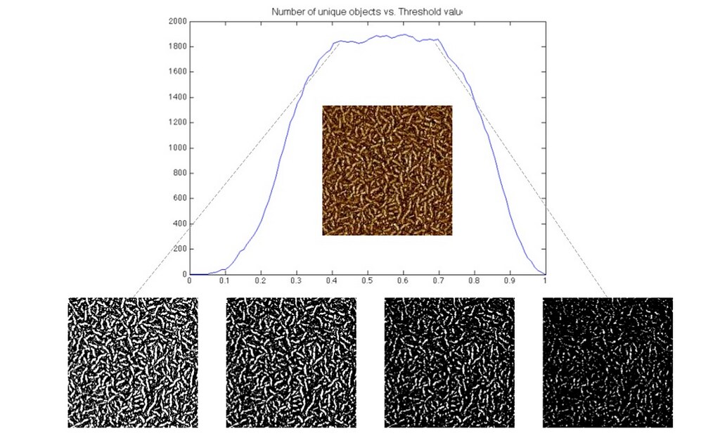For details on the algorithm, see the Thresholding Post.

Although an improvement on the first thresholding effort, this algorithm still used a single threshold value for each image. A single value threshold method fails because the pixel intensities associated with a fiber vary even across single AFM image.

Determining Fiber Orientation

regionprops was used to fit an ellipse to each connected component obtained from the previous thresholding to determine the orientation of that fiber. To see a proof of concept for this method visit the Fiber Orientation Post

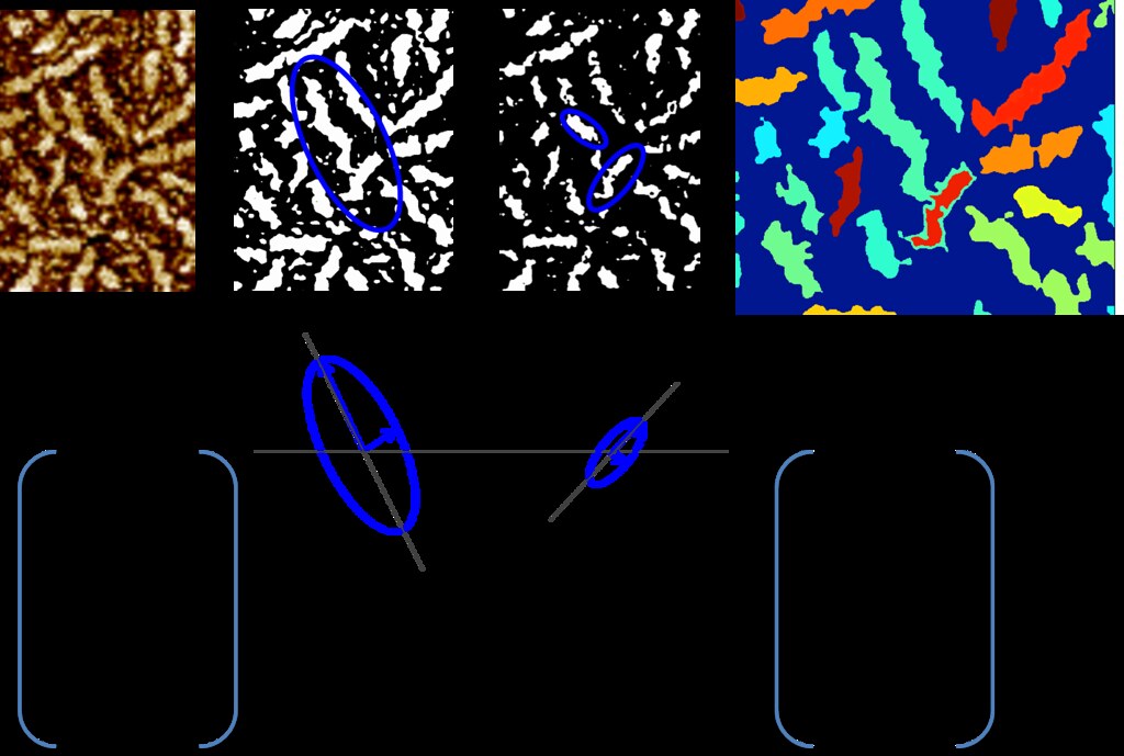
Overlapping fiber, especially those in completely different directions will contaminate the orientation calculation. The image below shows a case where the ellipse fit to the connected component in green will choose the green vector to calculate the orientation of the fiber. This orientation is incorrect for both fibers.

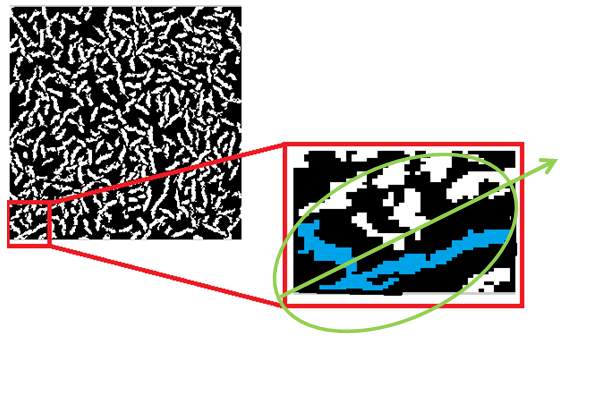
This issue is primarily caused by insufficient thresholding. Attempts were made to separate such connected fibers using tools like erode in matlab. We also attempted to identify orientation despite the connectivity using hough transformations. Both attempts were unsuccessful.

Orientation Informed Fiber Identification

The final and most successful attempt at image segmentation combined all lessons learned from previous attempts. The algorithm involves applying a range of threshold values to a single image. For each thresholded image, two matrices were calculated. The values in the matrices correspond to pixels in the image. The first matrix identified the orientation of the fibers. The second matrix identified the confidence with which the orientations belong to a fibular region. 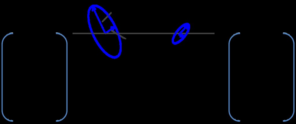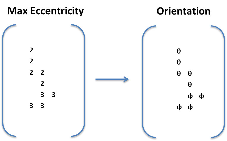To calculate these matrices, for each pixel, if the pixel was a part of a connected component, regionprops was used to fit an ellipse to the connected component. The vector associated with the major axis of the ellipse was used to determine orientation. The eccentricity of the ellipse, defined as the ratio of the major axis to the minor axis, to determine the extent to which the region was fiber like. The higher the eccentricity, the more likely that the region was a fiber. This portion of the algorithm is summarized in the figures below.

Next the algorithm finds the maximum confidence across all thresholds and takes their corresponding angles.

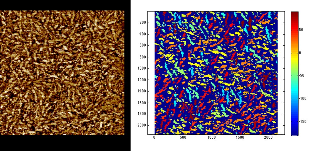
This algorithm allows us to identify individual fibers and their corresponding orientation as shown below: 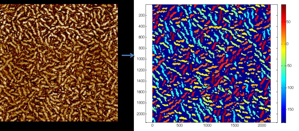Here the dark blue represents the amorphous phase, and the fibers are color coded according to their angle off of the horizontal. The portion of the color bar at right from -90 to 90 degrees encompasses the fiber angles.

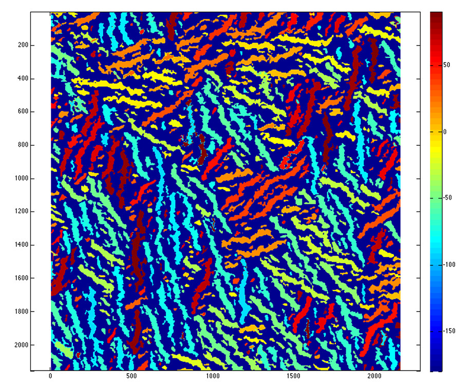
The algorithm works even for excessively noisy images such as:

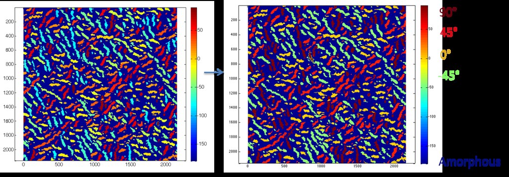
The final result can be used to determine useful features of the microstructure such as average fiber length. Other informative insights can be gained from visualization of fiber orientation. For example, the image below shows that fibers tend to form in clumps of 3 or four and have long range order.

More details about the algorithm can be found at its original post.

This algorithm has also been made available for public use with the help of Tony Fast.

Spatial Statistics

The range of orientations found for the fibers in each microstructure were binned into five states as shown below.

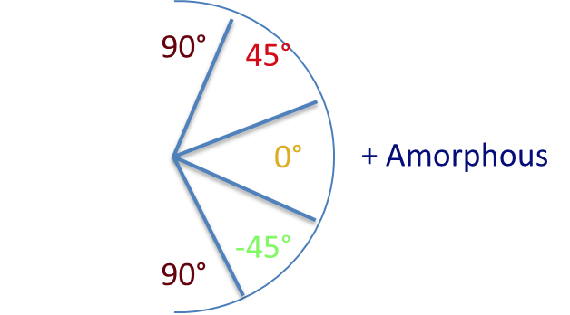
With five possible microstates ( 90 degrees, 45 degrees, -45 degrees, 0 degrees, amorphous), the spatial statistics matrix is 5x5, where each entry represents a matrix of either autocorrelation or cross correlation of microstates.

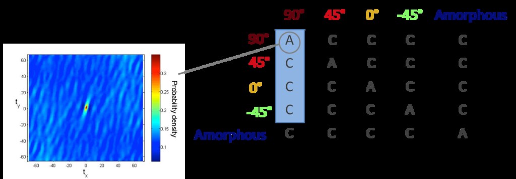
However, only four of the correlations are independent. Therefore, we generate these four spatial statistic matrices for all of our images.

The plot below shows the spatial statistics for a 90 degree, 90 degree oriented fiber autocorrelation for a single AFM image.

The highest intensity of 0.08 indicates that for this particular device, the area fraction of vertically oriented fibers is 8%. The green arrows on the AFM image show a few of these vertically oriented fibers. The light blue color on the spatial statistics heat map corresponds to 3%, indicating that 3% of vectors [0,55] have both their head and tail in a fiber.

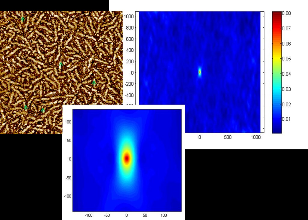
The plot below shows the spatial statistics for a 90 degree, 90 degree oriented fiber autocorrelation for a different AFM image.

Here we find that area fraction of vertically oriented fibers is similar to the previous device, yet the percent of vectors [55.0] that have both head and tail in a fiber is less, indicating shorter vertically oriented fibers, possibly non-fibrilar.

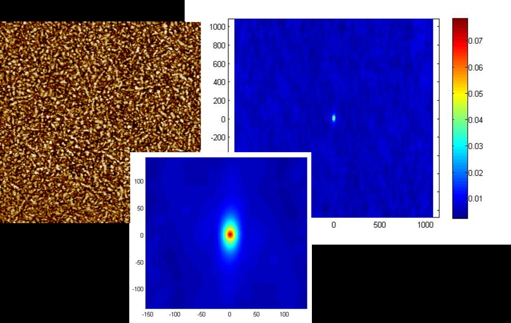
Similar analysis can be performed for the cross correlations.

Dimensionality Reduction

Principle Component Analysis (PCA) was performed on the combined four spatial statistics. Here we show the 90°/90° autocorrelation portion of the first principal component. Just as in spatial statistics, the x-y coordinates still correspond to vectors, but the intensities now indicate degrees of variance over the set of images.

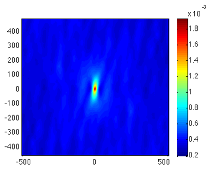
We find that the zero vector varies the most over the image set. This is the area fraction of 90° fibers. We also find that vertically oriented vectors vary a lot over the image set. This is indicative of fiber length. We find that spatial statistics combined with PCA objectively identified fiber length as a key feature of the dataset.

We can now analyze the data in Principle Component (PC) state as shown below.

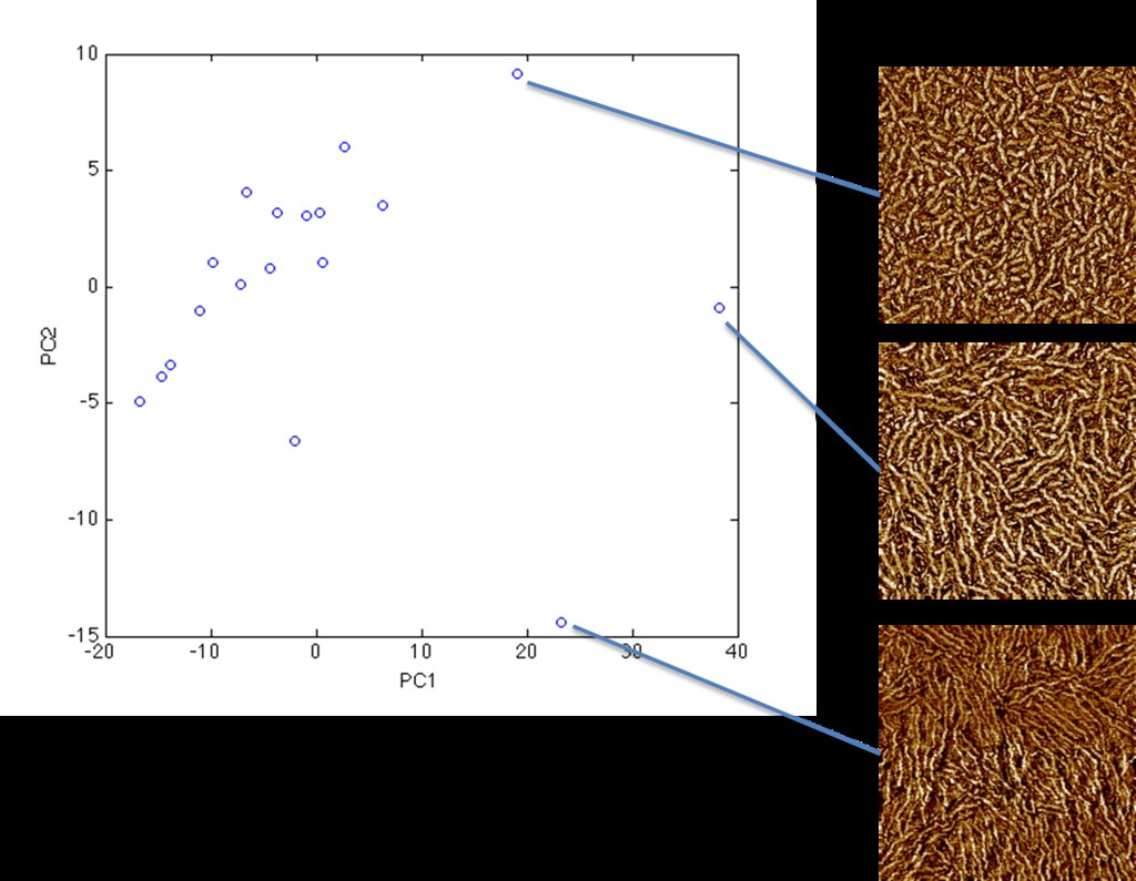
PCs 1 and 2 seem to capture some combination of fiber length, density, and thickness.

The Structure-Property Relationship

Multiple regression of measured mobilities (Y) vs. scores in the first four PCs (X) was performed to obtain µ = f( structure ) The cross-validated mean average error (CVMAE) is shown in the table below for range of polynomial order and principle components.

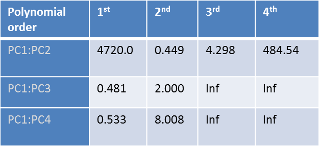
The best fit was obtained based the results of the above Leave-One-Out Cross Validation error to be a 2nd order polynomial in first two PC scores.

µ = B0 +B1 x PC1 score + B2 x PC2 score + B3 x PC1 Score x PC2 score + B4 x PC1 score ^2 + B5 x PC2 score ^2

where B = [-0.0003;0.0007;2.13e-05;0.0336;2.82e-05;-6.77e-05]

A similar approach was used to determine the best fit for mobility vs fiber length. The plot below shows predicted mobility (using PCs and Fiber Length ) vs measured mobility for all devices studied.

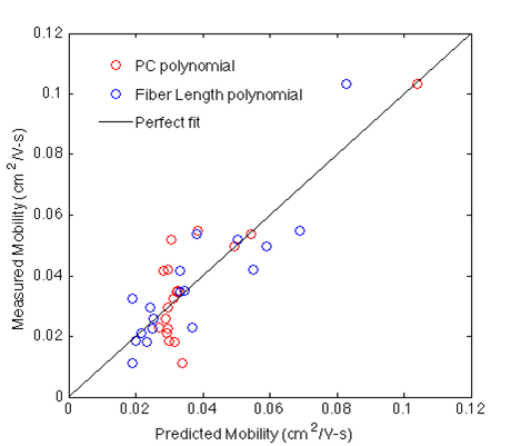
We find that while fiber length can be used to predict mobility, a structure-property relationship based on spatial statistics performs especially well on high-mobility devices. However, this method fails for devices with high area fraction, non-fibrilar samples.

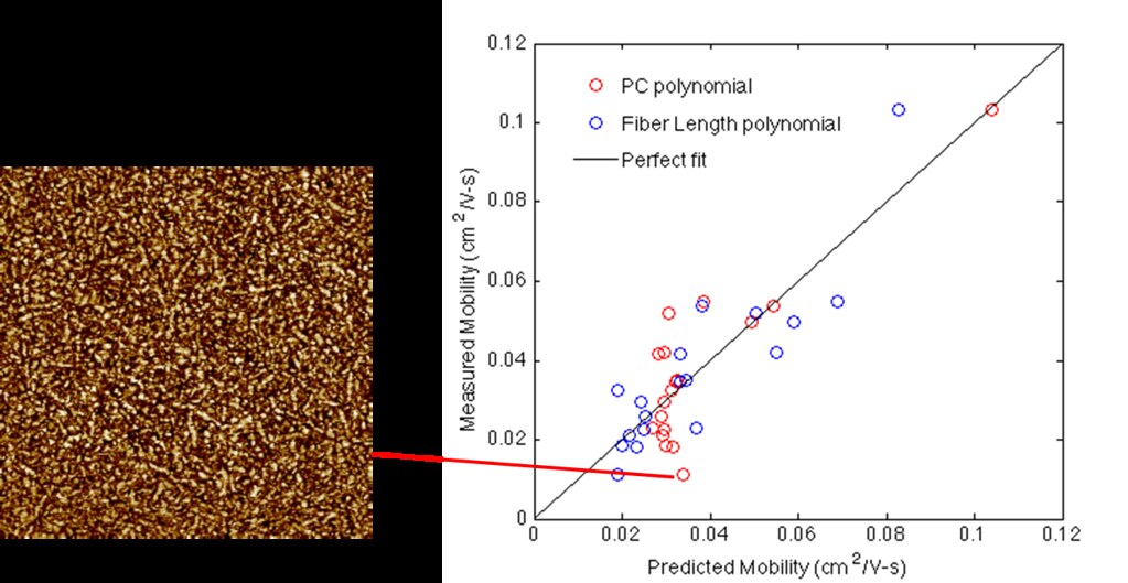
However, we find that using spatial statistics combined with PCA is an objective and successful method for defining a functional structue-popety relationship.

Collaboration

Throughout the semester we collaborated with classmates in a variety of ways, most noteworthy of these collaborations were:

1. Outside of class brainstorming meeting with Geet Lahoti and Alicia White to discuss possible segmentation methods.

2. Providing a publically available version of our segmentation method.

3. Providing a tutorial post on our website for setting of Swift Stack

To successfully complete our project, we also had to extensively collaborate with members of the Reichmanis Group. This was done through multiple presentations about the benefits of applying spatial statistics analysis and PCA to the dataset, updates about the progress of the project, and efforts to insure privacy of the data.

Team Dynamics

While each group member had specific tasks, the team dynamics relied heavily on consistent coding meetings and brainstorming sessions. In the past semester, the team has invested over 30 hours in collaborative work meetings outside of class time and post class discussions.

For efficiency, tasks were often performed separately and communicated with email, flickr, and dropbox.

Main Responsibilities

Nils Persson :

-Writing, debugging and polishing final codes used for data analysis. -Gather experimental results from collaborator.

Dalar Nazarian:

-Experimenting with alternative algorithms. -Maintaining group website and preparing posts.

Summary

• A robust image segmentation procedure was developed for AFM tapping-mode data
• Spatial statistics objectively identified features that we knew to be important, along with others that were not readily apparent
• We learned that our fibers tend to come in clumps, which provided valuable information about the underlying polymers’ morphology
• Our analysis yielded a predictive structure-property relationship from AFM data for electronic properties, something that has not been thoroughly quantified in the past
• The class has also informed our future experimental design. Future work is anticipated to include local structure and property measurement through AFM at higher resolutions and with more samples per device.

Refences

• J. A. Lim, F. Liu, S. Ferdous, M. Muthukumar, and A. L. Briseno, Mater. Today, 2010, 13, 14–24.
• R. Noriega, J. Rivnay, K. Vandewal, F. P. V Koch, N. Stingelin, P. Smith, M. F. Toney, and A. Salleo, Nat. Mater., 2013, 12, 1038–44.
• S. Himmelberger, K. Vandewal, Z. Fei, M. Heeney, and A. Salleo, Macromolecules, 2014, 47, 7151–7157.
• Y.-K. Lan and C.-I. Huang, J. Phys. Chem. B, 2009, 113, 14555–64.
• J.-C. Bolsée, W. D. Oosterbaan, L. Lutsen, D. Vanderzande, and J. Manca, Adv. Funct. Mater., 2013, 23, 862–869.